What are Your Chances of Winning Highlow?

Just like many Gen Z friend groups, my friends and I have a Discord server. We mainly use it for communication when we play video games together. But we also have some random channels - one of these is the “pancake” channel, where we collect, earn, and gamble a fake digital currency (pancakes) using a “pancake bot”. There are typical gambling games like blackjack and slots, for which much ink has been spilled concerning probability and statistics-informed strategies for winning. I have no more than a terribly basic understanding of those games. However, one of the pancake games is called with a command “p! highlow”. I choose to just call the game “Highlow”. There is no bet involved, so it’s not gambling, but you do earn pancakes if you win. 20 of them, to be exact. So the stakes are SUPER high.

Here’s how it works: a random integer from 1 to 100 is generated. The player must then decide whether an additional randomly generated integer from 1 to 100 (excluding the first one) will be higher or lower. After this, a new number is generated, and if the player is correct, they win the game (and 20 pancakes). Otherwise, they don’t lose or gain any pancakes.

It’s a straightfoward game. The best strategy for winning is intuitive - if our first number (let’s call it $n_1$) is 50 or below, we should select “high” since there are more numbers above $n_1$ than below (between 1 and 100). Otherwise, we should select “low”. The approximate chance of winning (given we know $n_1$) is also straightforward to see - if $n_1$ is 34, then you have around a 66 percent chance of winning (one percent for each number above 34 and at most 100), while a draw of 82 yields around an 81 percent chance of winning (one percent for each number below 82 and at least 1). We’ll figure out the exact percentages later, but the big idea is: The further your number is from the middle, the better your chances of winning.

This got me thinking - we know the chance of winning given our first draw, but what is the chance of winning the game overall, before we are given a number in the first place? This question was a bit harder to answer, but it was fun to figure out and also let me practice some of my data/programming skills, so I thought it would be cool to share! My goal was to write for an audience that includes people who are not super well-versed in statistics, so I’ve included explanations and definitions in places I thought would be helpful. Let’s dive in!

First… some Probability

Probability of winning given $n_1$

Earlier, I mentioned that finding the chance of winning given our first number ($n_1$) was straightforward. Let’s go over the math. Once $n_1$ is selected, the next number (we’ll call it $n_2$) MUST be distinct from $n_1$. This means there are 99 possibilities for $n_2$. If we guess “high”, then the chance of winning is equal to the number of outcomes higher than $n_1$ divided by 99. This will be greater than 50% as long as the number of outcomes higher than $n_1$ is at least 50. From this, we see what our intuition told us: if $n_1$ is 50, there are 50 outcomes above $n_1$ versus 49 below. If $n_1$ is 51, there are 50 outcomes below $n_1$ versus 49 above. So we have a rule:

$n_1 < 51$ $\Rightarrow$ guess “high”

otherwise $\Rightarrow$ guess “low”

Choosing this way guarantees a chance of winning of at least 50/99 = 50.5%, with the chance growing as $n_1$ increases or decreases.

Probability of winning overall

We understand how to find the chance of winning if we know $n_1$. But how can we find out the probability of winning the game before we know $n_1$? In other words, what percentage of attempts at this game should we expect to win? We can call this the overall probability or average probability of a win. To answer this, we will learn (or review) some probability theory and use the law of total probability.

In this game, there are 100 equally likely possibilities for $n_1$. For each possibility, the player can choose either “high” or “low”. Let’s assume that the player only chooses the option which gives them the best chance at winning. In this case, after $n_1$ is selected, there are two possible outcomes: a win or a loss. This means we have exactly 198 scenarios: 2 for $n_1$ = 1 or $n_1$ = 100, where we have a win. For $2 \leq n_1 \leq 99$, we have either a win or a loss, so for 98 numbers, each with 2 possible outcomes, we have $98 \cdot 2 = 196$ outcomes. In statistics, we call the set of all possible outcomes the sample space, which we can call $S$.

We can break this space $S$ up into groups, or subsets; for example, let’s group together outcomes with a common $n_1$. In other words, the outcomes {$n_1$ and win} and {$n_1$ and loss} would be in the same subset, and they actually constitute the entire subset, since these are the only possible outcomes given $n_1$. Let’s call these sets $B_n$, of which there are 100 for each possible $n_1$. These sets do not overlap, and they constitute the entire sample space $S$ - this means they form what we call a partition of the sample space. Besides this partition into sets $B_n$, we might also make a different subset of all the winning outcomes in $S$ - let’s call this subset $W$. This would include the outcomes {2 and win}, {3 and win}, {4 and win}, and so on.

Using this information, we can use the law of total probability. In English, it states that if we have a partition with $k$ elements of a sample space $S$ (where each subset in the partition has a nonzero probability), and we have some event A that is a subset of $S$, then the probability of A happening is equal to the sum of joint probabilities $A$ AND $B_i$ (for each element $B_i$ of the partition). In symbols, we have

\[P(A) = \sum_{i=1}^{k} P(A | B_i)P(B_i)\]

$P(A)$ represents the probability of event A, while $P(A \mid B_i)$ represents the probability of $A$ given the event $B_i$ has occurred.

In our problem, we have a partition of $S$, namely {$B_1$, $B_2$, … , $B_{100}$}, and a subset $W \subset S$. Plugging these in to the equation gives us

\[P(W) = \sum_{i=1}^{100} P(W|B_i)P(B_i)\]

In other words: To find the probability of winning the game, we must find (for every possible $n_1$) the probability of winning given a draw of $n_1$ AND drawing $n_1$ in the first place, then summing all 100 of these probabilities. For example, consider $n_1 = 1$. The probability of winning given a draw of 1 is 100%, while the probability of drawing a 1 is 1%. So, the probability of the outcome {1 and win} is 1%. Now consider $n_1 = 25$. The probability of winning given a draw of 25 is $\frac{100-25}{99} = 75.76\%$, while the probability of drawing a 25 is 1%. Thus, the probability of the outcome {25 and win} is approximately 0.76%. Intuitively, adding up these probabilities makes sense: We are simply finding the probability of {$n_1$ and win} for all $n_1$. Each of these events has no overlap (since more than one $n_1$ cannot be drawn) and constitutes all of the winning events, meaning we just have to sum their probabilities to get the overall probability of winning the game.

Alternatively, since each $B_i$ is equally likely, each $P(B_i)$ is equal. So we can treat this term in our formula as a constant and pull it out:

\[P(W) = P(B_i)\sum_{i=1}^{100} P(W|B_i)\]

But $P(B_i) = \frac{1}{100}$ for all $i$, so we see that we are actually computing a regular old arithmetic average (mean):

\[P(W) = \frac{\sum_{i=1}^{100} P(W|B_i)}{100}\]

Hence the term average probability; the general law of total probability is essentially a weighted average, where the weight is $P(B_i)$. For our problem, we have a special case where each probability is equally weighted. I took advantage of this when calculating our magic number with Google Sheets:

Calculating the average probability of winning highlow

In Google Sheets, I placed each $n_1$ from 1 through 100 in column A. Column B calculates $P(W \mid B_n)$ with the simple formula =(100-A2)/99 for $n_1 \le 50$, and =(A52-1)/99 for $n_1 \ge 51$. In Column C, I took the difference $1 - P(W \mid B_n)$ to get the probability of losing given a draw of $n$ (more on that later). I then calculated the average of column B, which yielded our magic number $P(W)$:

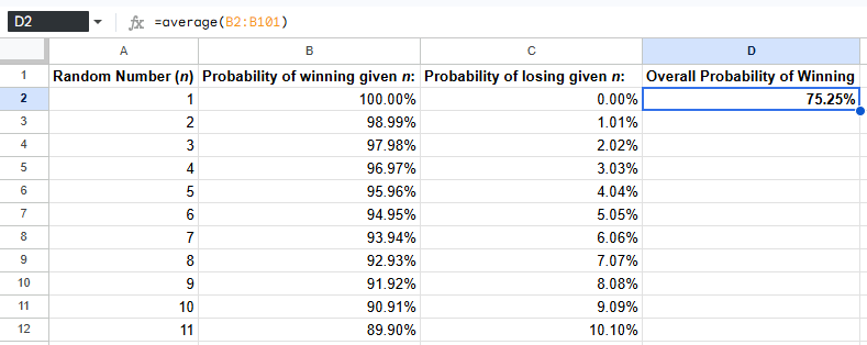
We can see that the average probability of winning highlow is approximately 75.25%. So, one should expect to win this game about $\frac{3}{4}$ of the time.

Another interpretation of this result is that if we were to make a set diagram of all the possibilities (where the probability of each event is scaled by its likelihood), about 75% of the area would be covered by winning outcomes. While I didn’t technically create a set diagram, I thought it would be a cool idea to create a visual with the same effect. To this end, I created a stacked bar chart in Google Sheets. Each bar represents an $n_1$ value (from 1 to 100). The bar is broken up proportionally into a blue area representing win probability and a red area representing loss probability. If we condense the chart to cover the area of a square, we can imagine this square as divided into four congruent isosceles triangles (by the two diagonals, shown below as orange lines). We then see that the top triangle which makes up approximately one fourth of the area of the square coincides with the area of the square covered by red:

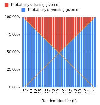
This is consistent with our math, which says that we have about a 25% chance of losing the game when we play. The graph also represents how one is likelier to win the closer one’s $n_1$ is to the extremes, 1 and 100, while a draw closer to 50 is less desireable, creating a symmetric “V” shape.

Empirical Testing with Python

If you flip a fair coin, it has a 50 percent chance of being heads or tails. But if you flip it three times, you have a 12.5 percent chance of flipping three heads or three tails in a row. In either case, the experimental probability of flipping heads or tails would be 100%, which does not reflect the expected or average probability. On the other hand, if you flip a coin 100 times, or even 1000 times, the proportion of heads to tails will be much closer. This is known as the law of large numbers. The more a random experiment is conducted, the closer the experimental probability of a result approaches the expected probability.

If we play 5 games of highlow, maybe we will win all of them, or only two of them. But if our math is right, then the more games of highlow we play, the closer we should get to winning 75% of them. We can test this out, and I did by writing a short Python program that plays highlow any number of times and plots the win rate as the attempts increase:

import random as rd
import matplotlib.pyplot as plt

# The following list allows us to track the win rates and plot them.
win_rates_over_time = []

# This function takes in a desired number of attempts at the game
# (with strategically correct guesses) and returns the win rate as a
# percentage rounded to three decimal places.

def highlow(x):
    # i tracks the number of attempts.
    i = 0
    wins = 0
    
    while i < x:
        i += 1
        n1 = rd.randint(1, 100)
        if n1 <= 50:
            guess = "High"
        else: guess = "Low"
        
        n2 = rd.randint(1,100)
        # The following while loop prevents n_2 from equalling n_1.
        while n2 == n1:
            n2 = rd.randint(1, 100)
        
        if n2 > n1:
            answer = "High"
        else: answer = "Low"
        
        if guess == answer:
            wins += 1
    win_rate = round(((wins/x)*100), 3)
    win_rates_over_time.append(win_rate)
    return win_rate

# The code below runs highlow "max_attempts" times (adjusting max_attempts will
# automatically adjust the plot range and when the win rate is printed to avoid
# excessive printing at high max_attempt numbers).
attempts = 1
max_attempts = 10
while attempts <= max_attempts:
    if attempts % (max_attempts/10) == 0:
        print(f"for {attempts} attempt(s), the win rate is {highlow(attempts)}%")
    else: 
        highlow(attempts)
    attempts += 1

# The following code plots win rates as the number of attempts increases.
plt.plot(range(1, (max_attempts + 1)), win_rates_over_time, linewidth=0.7)
plt.xlabel("Number of Attempts")
plt.ylabel("Win Rate (%)")

plt.title("Win Rate vs Attempts")
plt.axhline(y=75.25, linestyle='--', label='Expected Win Rate (~75.25%)')

plt.ylim(bottom=0)
plt.legend()

plt.show()

As noted in the code, the max number of attempts can be adjusted by changing the value of max_attempts. Here is a result for up to 10 attempts, with the expected win rate as a dotted line:

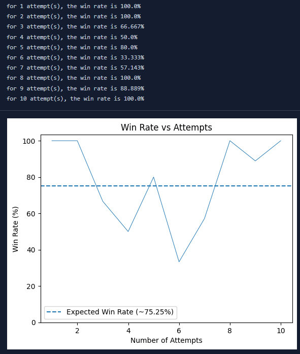
As expected, we have a very wide range of win rates, including ones below 40% for as many as six attempts. With this information, it would be very difficult to determine what the average win rate should be. Let’s bump the number up to 100 trials:

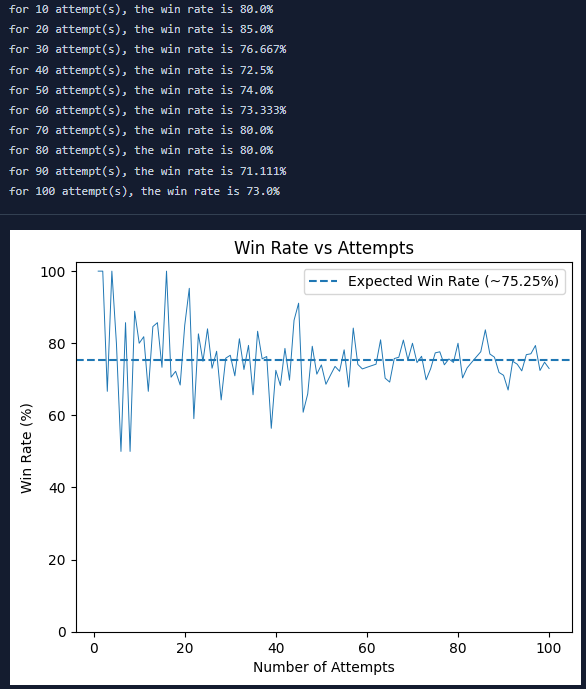
Now we are beginning to see a signal. There’s a lot of noise at first, but if we sample the win rate every tenth iteration (as shown above the graph), we remain pretty consistently in the 70-80 percent range. Now consider 1,000 and 10,000 attempts respectively:

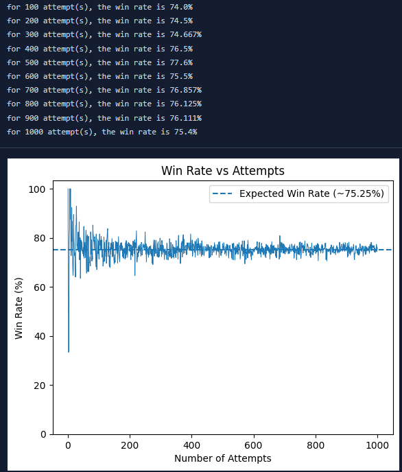
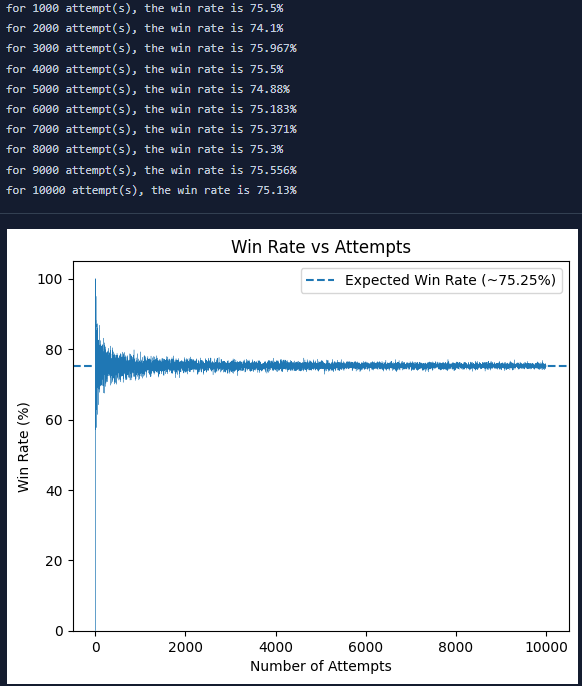
For 10,000 attempts, we see that every thousandth attempt 74 and 76 percent, a pretty tight range. We can clearly see the win rates converging roward the expected win rate of 75.25%. We haven’t proven the law of total probability in a formal sense (go see a mathematical statistics textbook for that), but we have some anecdotal evidence that it works!

Conclusion

Using the law of total probability, we were able to find the expected win rate for the game “highlow”. We were then able to see this rate as a share of the area of a square and finally test our findings empirically with the help of Python. As for future directions, I’m sure I could begin with trimming the code and making it more efficient/editable. This could allow for higher maximum trial counts. Additionally, I could edit the code to include user inputs so that anyone could run the program, plug in the desired numbers, and produce any number of custom charts.

What started as random curiosity has ended up as great practice in statistics, probability, programming, and data analytics. I am glad to share this with the world and of course would love to hear any feedback!

Thank you so much!

I appreciate any comments and tips! Check out my LinkedIn and send a DM or comment on my post about this project. Thanks for getting this far!